Radial Trees in Tableau by Chris DeMartini
/
Before we get into it, I wanted to include a shameless plug for my fellow DataBlick'ers upcoming sessions at the Tableau Conference. Be sure to check them out if you are heading that way!
- Tableau Minority Report: A Tableau UX of the Future (Anya A'Hearn, Allan Walker and Jeffery Shaffer)
- Mapbox Fabulousness in Tableau: Lessons from a Zen Master (Anya A'Hearn and Allan Walker)
- Drawing with Tableau: Ridiculous Visualizations from a Zen Master (Noah Salvaterra)
- Tableau on a Shoestring: Successful Deployment on a Tiny Budget (Jonathan Drummey)
This is an incremental post to navigating your family tree from a few months back. This builds off of that visualization technique to manipulate the tree into a radial view. Also, as with the original, the tree is 100% dynamic and you can reset each node in the tree as the root node, toggle between tree views as well as change the API you are analyzing.
What is the benefit of a radial tree? As I discussed in my recent Tableau Fringe Festival presentation, it is really a give and take. Overall, it is probably easier to follow a path through a horizontal/vertical tree diagram. However, as your data volume and hierarchy levels increase, you will ultimately run out of space on your screen. That is where the radial tree can add value. With the root node as the center of the viz, and each level of the hierarchy increasing in diameter, you ultimately have more viz real estate to work with as you dig deeper into your hierarchy.
The use case I leveraged for this post is taking a look at the Tableau JS API class/object structure. I chose this in order to more easily navigate the Tableau JS API objects available to us all. I also incorporated the Flare API class structure for comparison purposes. Lastly, this effort was inspired by a similar D3 implementation.
To arrive at the radial tree, I started with the vertical hierarchy tree, a carbon copy of the family tree post discussed above. From this point it was just a matter of taking this tree and manipulating it into a circle. Honestly, I spent way more time than needed trying to figure out how to do this with a whole new set of calculations. If it is not broken, don't fix it! Once I settled on leveraging my existing tree and just manipulating it into a radial version, I needed a total of five additional calculated fields to bend my vertical tree into a radial tree.
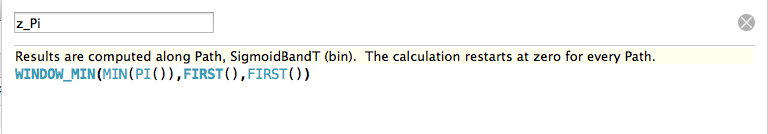
Calculation 1: A window table calculation to apply PI() across our data densification technique.
Calculation 2: A level of detail calculation that will return the maximum node placement across the entire population. This result is than applied to the same table calculation as our other fields. LOD made this so much easier!

Calculations 3 and 4: This is the trickiest part. Leveraging our previous sigmoid curve function we are going to create x/y coordinates in a circle. One of the main things we need to know is where our points are in relation to one another. To figure this out, I used a percentage of maximum node technique. This is best described by the below images and I once again leveraged the handoff-map created by Joe Mako.


In this example the left most node is closest to 0% and the right most node is closest to 100%. We adapt that to a circle implementation shown on the right, via the below calculations.


Quick side note: While in the process of implementing these fields, I came across this result, not very meaningful, but reminded me of star wars a bit…

Calculation 5: This last calculation is just an adaptation of Jeffery Shaffer’s “Points” calculation, leveraging our radial field created above instead of our linear field.

From here we just need to place the respective calculations on their corresponding shelves and we now see our radial tree! Compare the two versions below and you will note identical use of our rows/columns shelves (inversed) between the two implementations.


There have been a couple requests for the underlying excel files, you can download them here.
